Examples
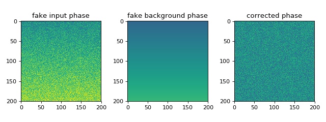
Simple phase
This example illustrates the simple usage of the
qpimage.QPImage class for reading and
managing quantitative phase data. The attribute QPImage.pha yields
the background-corrected phase data and the attribute
QPImage.bg_pha yields the background phase image.
 1import matplotlib.pylab as plt
 2import numpy as np
 3import qpimage
 4
 5size = 200
 6# background phase image with a tilt
 7bg = np.repeat(np.linspace(0, 1, size), size).reshape(size, size)
 8# phase image with random noise
 9phase = np.random.rand(size, size) + bg
10
11# create QPImage instance
12qpi = qpimage.QPImage(data=phase, bg_data=bg, which_data="phase")
13
14# plot the properties of `qpi`
15plt.figure(figsize=(8, 3))
16plot_kw = {"vmin": -1,
17           "vmax": 2}
18
19plt.subplot(131, title="fake input phase")
20plt.imshow(phase, **plot_kw)
21
22plt.subplot(132, title="fake background phase")
23plt.imshow(qpi.bg_pha, **plot_kw)
24
25plt.subplot(133, title="corrected phase")
26plt.imshow(qpi.pha, **plot_kw)
27
28plt.tight_layout()
29plt.show()
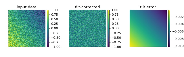
Background image tilt correction
This example illustrates background tilt correction with qpimage.
In contrast to the ‘simple_phase.py’ example, the known background data
is not given to the qpimage.QPImage
class. In this particular example, the background tilt correction
achieves an error of about 1% which is sufficient in most quantitative
phase imaging applications.
 1import matplotlib.pylab as plt
 2import numpy as np
 3import qpimage
 4
 5size = 200
 6# background phase image with a tilt
 7bg = np.repeat(np.linspace(0, 1, size), size).reshape(size, size)
 8bg = .6 * bg - .8 * bg.transpose() + .2
 9# phase image with random noise
10rsobj = np.random.RandomState(47)
11phase = rsobj.rand(size, size) - .5 + bg
12
13# create QPImage instance
14qpi = qpimage.QPImage(data=phase, which_data="phase")
15# compute background with 2d tilt approach
16qpi.compute_bg(which_data="phase",  # correct phase image
17               fit_offset="fit",  # use bg offset from tilt fit
18               fit_profile="tilt",  # perform 2D tilt fit
19               border_px=5,  # use 5 px border around image
20               )
21
22# plot the properties of `qpi`
23fig = plt.figure(figsize=(8, 2.5))
24plot_kw = {"vmin": -1,
25           "vmax": 1}
26
27ax1 = plt.subplot(131, title="input data")
28map1 = ax1.imshow(phase, **plot_kw)
29plt.colorbar(map1, ax=ax1, fraction=.046, pad=0.04)
30
31ax2 = plt.subplot(132, title="tilt-corrected")
32map2 = ax2.imshow(qpi.pha, **plot_kw)
33plt.colorbar(map2, ax=ax2, fraction=.046, pad=0.04)
34
35ax3 = plt.subplot(133, title="tilt error")
36map3 = ax3.imshow(bg - qpi.bg_pha)
37plt.colorbar(map3, ax=ax3, fraction=.046, pad=0.04)
38
39# disable axes
40[ax.axis("off") for ax in [ax1, ax2, ax3]]
41
42plt.tight_layout(pad=0, h_pad=0, w_pad=0)
43plt.show()
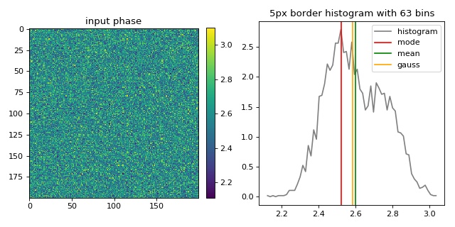
Background image offset correction
This example illustrates the different background offset correction methods implemented in qpimage. The phase image data contains two gaussian noise distributions for which these methods yield different background phase offsets.
 1import matplotlib.pylab as plt
 2import numpy as np
 3import qpimage
 4
 5size = 200  # the size of the image
 6bg = 2.5  # the center of the background phase distribution
 7scale = .1  # the spread of the background phase distribution
 8
 9# compute random phase data
10rsobj = np.random.RandomState(42)
11data = rsobj.normal(loc=bg, scale=scale, size=size**2)
12# Add a second distribution `data2` at random positions `idx`,
13# such that there is no pure gaussian distribution.
14# (otherwise 'mean' and 'gaussian' cannot be distinguished)
15data2 = rsobj.normal(loc=bg*1.1, scale=scale, size=size**2//2)
16idx = rsobj.choice(data.size, data.size//2)
17data[idx] = data2
18# reshape `data` to get a 2D array
19data = data.reshape(size, size)
20
21qpi = qpimage.QPImage(data=data, which_data="phase")
22
23cpkw = {"which_data": "phase",  # correct the input phase data
24        "fit_profile": "offset",  # perform offset correction only
25        "border_px": 5,  # use a border of 5px of the input phase
26        "ret_mask": True,  # return the mask image for visualization
27        }
28
29mask = qpi.compute_bg(fit_offset="mode", **cpkw)
30bg_mode = np.mean(qpi.bg_pha[mask])
31
32qpi.compute_bg(fit_offset="mean", **cpkw)
33bg_mean = np.mean(qpi.bg_pha[mask])
34
35qpi.compute_bg(fit_offset="gauss", **cpkw)
36bg_gauss = np.mean(qpi.bg_pha[mask])
37
38bg_data = (qpi.pha + qpi.bg_pha)[mask]
39# compute histogram
40nbins = int(np.ceil(np.sqrt(bg_data.size)))
41mind, maxd = bg_data.min(), bg_data.max()
42histo = np.histogram(bg_data, nbins, density=True, range=(mind, maxd))
43dx = abs(histo[1][1] - histo[1][2]) / 2
44hx = histo[1][1:] - dx
45hy = histo[0]
46
47# plot the properties of `qpi`
48plt.figure(figsize=(8, 4))
49
50ax1 = plt.subplot(121, title="input phase")
51map1 = plt.imshow(data)
52plt.colorbar(map1, ax=ax1, fraction=.046, pad=0.04)
53
54
55t2 = "{}px border histogram with {} bins".format(cpkw["border_px"], nbins)
56plt.subplot(122, title=t2)
57plt.plot(hx, hy, label="histogram", color="gray")
58plt.axvline(bg_mode, 0, 1, label="mode", color="red")
59plt.axvline(bg_mean, 0, 1, label="mean", color="green")
60plt.axvline(bg_gauss, 0, 1, label="gauss", color="orange")
61plt.legend()
62
63plt.tight_layout()
64plt.show()
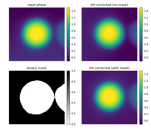
Masked background image correction
This example illustrates background correction with qpimage using a mask to exclude regions that do not contain background information.
The phase image of a microgel bead (top left) has two artifacts; there is a tilt-like phase profile added along the vertical axis and there is a second microgel bead in close proximity to the center bead. A regular phase tilt background correction using the image values around a frame of five pixels (see “background_tilt.py” example) does not yield a flat background, because the second bead is fitted into the background which leads to a horizontal background phase profile (top right). By defining a mask (bottom left image), the phase values of the second bead can be excluded from the background tilt fit and a flat background phase is achieved (bottom right).
 1import matplotlib.pylab as plt
 2import numpy as np
 3import qpimage
 4
 5
 6# load the experimental data
 7input_phase = np.load("./data/phase_beads_close.npz")["phase"].astype(float)
 8
 9# create QPImage instance
10qpi = qpimage.QPImage(data=input_phase,
11                      which_data="phase")
12
13# background correction without mask
14qpi.compute_bg(which_data="phase",
15               fit_offset="fit",
16               fit_profile="tilt",
17               border_px=5,
18               )
19pha_nomask = qpi.pha
20
21# educated guess for mask
22mask = input_phase < input_phase.max() / 10
23
24# background correction with mask
25# (the intersection of `mask` and the 5px border is used for fitting)
26qpi.compute_bg(which_data="phase",
27               fit_offset="fit",
28               fit_profile="tilt",
29               border_px=5,
30               from_mask=mask
31               )
32pha_mask = qpi.pha
33
34# plot
35fig = plt.figure(figsize=(8, 7))
36plot_kw = {"vmin": -.1,
37           "vmax": 1.5}
38
39ax1 = plt.subplot(221, title="input phase")
40map1 = ax1.imshow(input_phase, **plot_kw)
41plt.colorbar(map1, ax=ax1, fraction=.044, pad=0.04)
42
43ax2 = plt.subplot(222, title="tilt-corrected (no mask)")
44map2 = ax2.imshow(pha_nomask, **plot_kw)
45plt.colorbar(map2, ax=ax2, fraction=.044, pad=0.04)
46
47ax3 = plt.subplot(223, title="mask")
48map3 = ax3.imshow(1.*mask, cmap="gray_r")
49plt.colorbar(map3, ax=ax3, fraction=.044, pad=0.04)
50
51ax4 = plt.subplot(224, title="tilt-corrected (with mask)")
52map4 = ax4.imshow(pha_mask, **plot_kw)
53plt.colorbar(map4, ax=ax4, fraction=.044, pad=0.04)
54
55# disable axes
56[ax.axis("off") for ax in [ax1, ax2, ax3, ax3, ax4]]
57
58plt.tight_layout(h_pad=0, w_pad=0)
59plt.show()
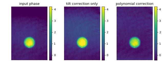
Background image 2nd order polynomial correction
This example extends the tilt correction (‘background_tilt.py’) to a second order polynomial correction for samples that exhibit more sophisticated phase aberrations. The phase background correction is computed from a ten pixel wide frame around the image. The phase data shown are computed from a hologram of a single myeloid leukemia cell (HL60) recorded using digital holographic microscopy (DHM) (see [SSM+15]).
 1import matplotlib.pylab as plt
 2import numpy as np
 3# The data are stored in a .jpg file (lossy compression).
 4# If `PIL` is not found, try installing the `pillow` package.
 5from PIL import Image
 6import qpimage
 7
 8edata = np.array(Image.open("./data/hologram_cell_curved_bg.jpg"))
 9
10# create QPImage instance
11qpi = qpimage.QPImage(data=edata, which_data="raw-oah")
12pha0 = qpi.pha
13
14# background correction using tilt only
15qpi.compute_bg(which_data=["phase"],
16               fit_offset="fit",
17               fit_profile="tilt",
18               border_px=10,
19               )
20pha_tilt = qpi.pha
21
22# background correction using polynomial
23qpi.compute_bg(which_data=["phase"],
24               fit_offset="fit",
25               fit_profile="poly2o",
26               border_px=10,
27               )
28pha_poly2o = qpi.pha
29
30# plot phase data
31fig = plt.figure(figsize=(8, 3.3))
32
33phakw = {"cmap": "viridis",
34         "interpolation": "bicubic",
35         "vmin": pha_poly2o.min(),
36         "vmax": pha_poly2o.max()}
37
38ax1 = plt.subplot(131, title="input phase")
39map1 = ax1.imshow(pha0, **phakw)
40plt.colorbar(map1, ax=ax1, fraction=.067, pad=0.04)
41
42ax2 = plt.subplot(132, title="tilt correction only")
43map2 = ax2.imshow(pha_tilt, **phakw)
44plt.colorbar(map2, ax=ax2, fraction=.067, pad=0.04)
45
46ax3 = plt.subplot(133, title="polynomial correction")
47map3 = ax3.imshow(pha_poly2o, **phakw)
48plt.colorbar(map3, ax=ax3, fraction=.067, pad=0.04)
49
50# disable axes
51[ax.axis("off") for ax in [ax1, ax2, ax3]]
52
53plt.tight_layout(w_pad=0)
54plt.show()
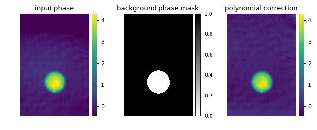
Object-mask background image correction
In some cases, using only the border of the phase image for background correction
might not be enough. To increase the area of the background image,
it is possible to mask only the cell area. The qpsphere package provides the convenience method
qpsphere.cnvnc.bg_phase_mask_for_qpi() which computes
the background phase mask based on the position and radius of an
automatically detected spherical phase object. The sized of the
mask can be tuned with the radial_clearance parameter.
Note that the various methods used in the examples for determining such a phase mask can be combined. Also note that before applying the method discussed here, an initial background correction might be necessary.
 1import matplotlib.pylab as plt
 2import numpy as np
 3# The data are stored in a .jpg file (lossy compression).
 4# If `PIL` is not found, try installing the `pillow` package.
 5from PIL import Image
 6import qpimage
 7import qpsphere
 8
 9edata = np.array(Image.open("./data/hologram_cell_curved_bg.jpg"))
10
11# create QPImage instance
12qpi = qpimage.QPImage(data=edata,
13                      which_data="raw-oah",
14                      meta_data={"medium index": 1.335,
15                                 "wavelength": 550e-9,
16                                 "pixel size": 0.107e-6})
17pha0 = qpi.pha
18
19# determine the position of the cell (takes a while)
20mask = qpsphere.cnvnc.bg_phase_mask_for_qpi(qpi=qpi,
21                                            r0=7e-6,
22                                            method="edge",
23                                            model="projection",
24                                            radial_clearance=1.15)
25
26# background correction using polynomial and mask
27qpi.compute_bg(which_data=["phase"],
28               fit_offset="fit",
29               fit_profile="poly2o",
30               from_mask=mask,
31               )
32pha_corr = qpi.pha
33
34# plot phase data
35fig = plt.figure(figsize=(8, 3.3))
36
37phakw = {"cmap": "viridis",
38         "interpolation": "bicubic",
39         "vmin": pha_corr.min(),
40         "vmax": pha_corr.max()}
41
42ax1 = plt.subplot(131, title="input phase")
43map1 = ax1.imshow(pha0, **phakw)
44plt.colorbar(map1, ax=ax1, fraction=.067, pad=0.04)
45
46ax2 = plt.subplot(132, title="background phase mask")
47map2 = ax2.imshow(1.*mask, cmap="gray_r")
48plt.colorbar(map2, ax=ax2, fraction=.067, pad=0.04)
49
50ax3 = plt.subplot(133, title="polynomial correction")
51map3 = ax3.imshow(pha_corr, **phakw)
52plt.colorbar(map3, ax=ax3, fraction=.067, pad=0.04)
53
54# disable axes
55[ax.axis("off") for ax in [ax1, ax2, ax3]]
56
57plt.tight_layout(w_pad=0)
58plt.show()
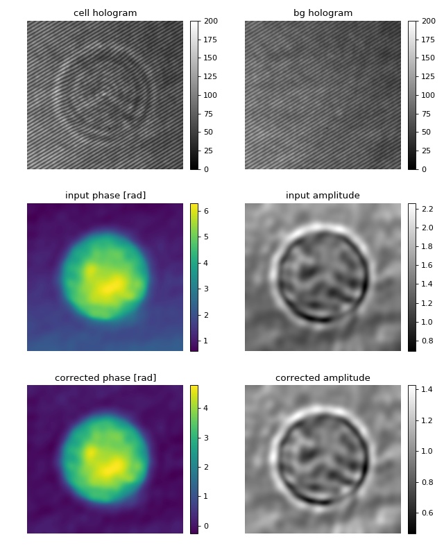
Off-axis hologram of a single cell
This example illustrates how qpimage can be used to analyze digital holograms. The hologram of a single myeloid leukemia cell (HL60) shown was recorded using digital holographic microscopy (DHM). Because the phase-retrieval method used in DHM is based on the discrete Fourier transform, there always is a residual background phase tilt which must be removed for further image analysis. The setup used for recording these data is described in reference [SSM+15], which also contains a description of the hologram-to-phase conversion and phase background correction algorithms which qpimage is based on.
 1import matplotlib
 2import matplotlib.pylab as plt
 3import numpy as np
 4import qpimage
 5
 6# load the experimental data
 7edata = np.load("./data/hologram_cell.npz")
 8
 9# create QPImage instance
10qpi = qpimage.QPImage(data=edata["data"],
11                      bg_data=edata["bg_data"],
12                      which_data="raw-oah",
13                      # This parameter allows passing arguments to the
14                      # hologram-analysis algorithm in qpretrieve.
15                      qpretrieve_kw={
16                          # For this hologram, the "smooth disk"
17                          # filter yields the best trade-off
18                          # between interference from the central
19                          # band and image resolution.
20                          "filter_name": "smooth disk",
21                          # Set the filter size to half the distance
22                          # between the central band and the sideband.
23                          "filter_size": 1/2
24                          }
25                      )
26
27amp0 = qpi.amp
28pha0 = qpi.pha
29
30# background correction
31qpi.compute_bg(which_data=["amplitude", "phase"],
32               fit_offset="fit",
33               fit_profile="tilt",
34               border_px=5,
35               )
36
37# plot the properties of `qpi`
38fig = plt.figure(figsize=(8, 10))
39
40matplotlib.rcParams["image.interpolation"] = "bicubic"
41holkw = {"cmap": "gray",
42         "vmin": 0,
43         "vmax": 200}
44
45ax1 = plt.subplot(321, title="cell hologram")
46map1 = ax1.imshow(edata["data"], **holkw)
47plt.colorbar(map1, ax=ax1, fraction=.046, pad=0.04)
48
49ax2 = plt.subplot(322, title="bg hologram")
50map2 = ax2.imshow(edata["bg_data"], **holkw)
51plt.colorbar(map2, ax=ax2, fraction=.046, pad=0.04)
52
53ax3 = plt.subplot(323, title="input phase [rad]")
54map3 = ax3.imshow(pha0)
55plt.colorbar(map3, ax=ax3, fraction=.046, pad=0.04)
56
57ax4 = plt.subplot(324, title="input amplitude")
58map4 = ax4.imshow(amp0, cmap="gray")
59plt.colorbar(map4, ax=ax4, fraction=.046, pad=0.04)
60
61ax5 = plt.subplot(325, title="corrected phase [rad]")
62map5 = ax5.imshow(qpi.pha)
63plt.colorbar(map5, ax=ax5, fraction=.046, pad=0.04)
64
65ax6 = plt.subplot(326, title="corrected amplitude")
66map6 = ax6.imshow(qpi.amp, cmap="gray")
67plt.colorbar(map6, ax=ax6, fraction=.046, pad=0.04)
68
69# disable axes
70[ax.axis("off") for ax in [ax1, ax2, ax3, ax4, ax5, ax6]]
71
72plt.tight_layout()
73plt.show()
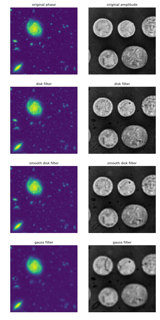
Filter choices for interferometric imaging
There are several parameters that influence the quality of phase and amplitude data retrieved from data recorded via interferometric techniques. This example demonstrates the advantages and disadvantages of three filtering stragies in qpimage. For more information, please have a look at the qpretrieve library.
Several observations can be made:
There appears to be a “bleed-through” of phase data into the amplitude data.
A (sharp) disk filter introduces ringing artifacts in the amplitude and phase images.
A smooth disk filter does not lead to such artifacts, but a dark halo is introduced around the coins in the amplitude image.
The amplitude reconstruction with the gaussian filter does not exhibit the dark halo but, due to blurring, reveals less details.
To correctly interpret the data shown, please note that:
This is a simulated hologram with no central band. For real data, the “filter_size” parameter also affects the reconstruction quality. Contributions from the central band can lead to strong artifacts. A balance between high resolution (large filter size) and small contributions from the central band (small filter size) usually has to be found.
It is not trivial to compare a gaussian filter with a disk filter in terms of filter size (sigma vs. radius). The gaussian filter takes into account larger frequencies and suppresses low frequencies. In qpimage, the actual gaussian filter size is chosen such that the resolution approximately matches that of the disk filter with a corresponding radius. In general however, the filter size parameter has to be examined when comparing the two.
There is an inherent loss of information (resolution) in the holographic reconstruction process. The side band is isolated with a low-pass filter in Fourier space. The size and shape of this filter determine the resolution of the phase and amplitude images. As a result, the level of detail of all reconstructions shown is lower than that of the original images.
 1import matplotlib.pylab as plt
 2import numpy as np
 3import qpimage
 4from skimage import color, data
 5
 6# image of a galaxy recorded with the Hubble telescope
 7img1 = color.rgb2gray(data.hubble_deep_field())[354:504, 70:220]
 8# image of a coin
 9img2 = data.coins()[150:300, 70:220]
10
11pha = img1/img1.max() * 2 * np.pi
12amp = img2/img2.mean()
13
14# create a hologram
15x, y = np.mgrid[0:150, 0:150]
16hologram = 2 * amp * np.cos(-2 * (x + y) + pha)
17
18filters = ["disk", "smooth disk", "gauss"]
19qpis = []
20
21for filter_name in filters:
22    qpi = qpimage.QPImage(data=hologram,
23                          which_data="raw-oah",
24                          qpretrieve_kw={"filter_size": .5,
25                                         "filter_name": filter_name})
26    qpis.append(qpi)
27
28fig = plt.figure(figsize=(8, 16))
29
30phakw = {"interpolation": "bicubic",
31         "cmap": "viridis",
32         "vmin": pha.min(),
33         "vmax": pha.max(),
34         }
35
36ampkw = {"interpolation": "bicubic",
37         "cmap": "gray",
38         "vmin": amp.min(),
39         "vmax": amp.max()
40         }
41
42numrows = len(filters) + 1
43
44plt.subplot(numrows, 2, 1, title="original phase")
45plt.imshow(pha, **phakw)
46
47ax2 = plt.subplot(numrows, 2, 2, title="original amplitude")
48plt.imshow(amp, **ampkw)
49
50for ii in range(len(filters)):
51    # phase
52    plt.subplot(numrows, 2, 2*ii+3, title=filters[ii]+" filter")
53    plt.imshow(qpis[ii].pha, **phakw)
54    # amplitude
55    plt.subplot(numrows, 2, 2*ii+4, title=filters[ii]+" filter")
56    plt.imshow(qpis[ii].amp, **ampkw)
57
58# disable axes
59for ax in fig.get_axes():
60    ax.axis("off")
61
62plt.tight_layout()
63plt.show()